2D Gaussian Splatting, SIGGRAPH 2024
Intro
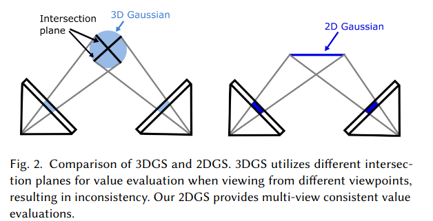
- 3DGS : Redering결과 Inconsistency한 depth발생, 왜냐하면 pixel ray사이의 intersection을 통해 gaussian value를 구하기 때문
- 2DGS : explicit ray-splat intersection 이용
- surface normal 정확하게 추출하면 mesh도 잘 구해짐
depth distortion
: 2D primitives에 집중해서 더 좁은 범위의 ray에 가우시안들이 분포하게 해줌
normal consistency
: rendered normal map과 rendered depth의 gradient 사이의 discrepancies 를 최소화함
두 개 regularaization term을 이용해서 smoother surface 구함
Contributions
- efficient differentiable 2D Gaussian Renderer
- surface recon을 위한 2가지 정규화 텀 소개 (depth distortion, normal consistency)
- sota Reconstruction & NVS result
1. Modeling
- normal = the steepest change of density
- better alignment with thin surfaces
- input = only a sparse calibration point cloud & photometric supervision
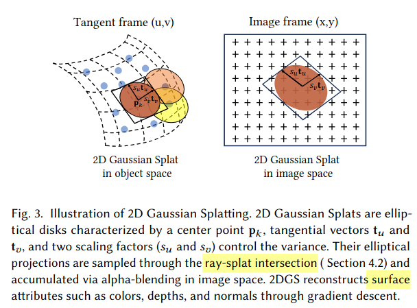
2D Gaussian Explicit Properties
- central point $p_k$
- two principal tangential vector $t_u, t_v$
scaling vector $S = (s_u, s_v)$
- primitive normal : $t_w = t_u \times t_v$
3x3 Rotation matrix $R = [t_u, t_v, t_w]$
- 2D Gaussian들은 local tangent plane에 정의됨
$P(u,v) = p_k + s_ut_uu + s_vt_vv =H(u,v,1,1)^T$ ⇒ world space에서 정의된 local tangent plane에서의 2D Gaussian point
where $H$ is the homogeneous transformation matrix, representing the geometry of the 2D Gaussian
$G($u$) = exp(-\frac{u^2+v^2}{2})$
$point - \mathrm{u} = (u, v)$
2. Splatting
- image space로 2D Gaussian들을 project하는 과정
- affine approximation of Perspective Transformation 이용
- Perspective transformation은 평행성이 지켜지지 않음, parallel한 line들이 소실점(vanishing point)에서 만남
한계점(선행 조건필요) :
center of the Gaussian이 정확해야하고,
center로부터의 거리가 멀어질수록 approximation error가 증가해야함
- homogeneous coordinate을 이용해서 완화된 해결방법 제안됨
2D Splat을 2D image plane에 projection한느 건 일반적인 2D-to-2D mapping in homogeneous coordinate이라고 할 수 있다
- $W$ : transformation matrix from World space to Screen space
Screen space에서의 projected points $\mathrm{x}$
$\mathrm{x} = (xz, yz, z, 1)^T = WP(u,v) = WH(u,v,1,1)^T$ 로 구해짐
- 2D Gaussian들을 rasterize하려면, inverse transfomation 인 $M= (WH)^{-1}$을 이용하는 방법이 있으나, 이 방법은 numerical instability함 특히 splat이 line segment(view가 옆면에서 보이는 상황인 경우, )에서 특히 결함이 많음
이 문제 해결위해 previous surface splatting rendering method들은 미리 정의된 predefined threshold을 이용해서 ill-conditioned transformation을 이용해왔음 (related work)
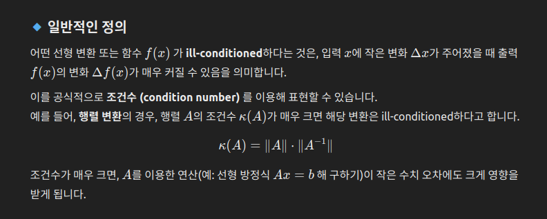
⇒ 모두 unstable함, 따라서 본 논문에서는 “Ray-Splat Intersection” 기반 방법을 제안
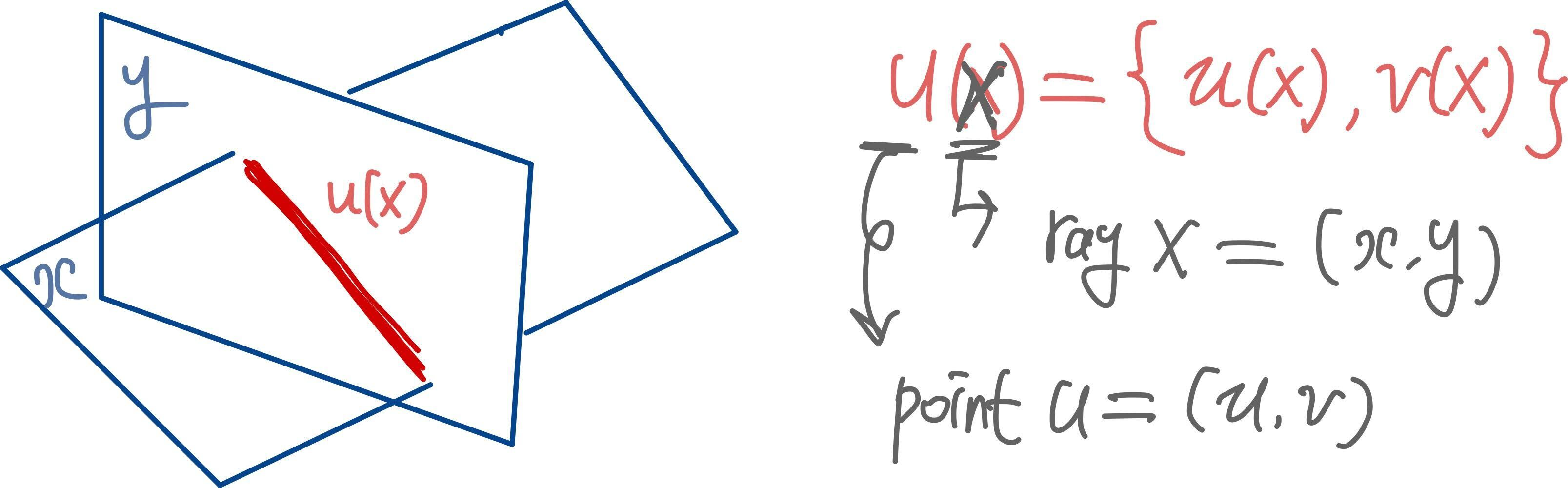
2-1. Ray-Splat Intersection
평행하지 않은 3가지 평면 (three non-parallel planes) 에서의 교점을 찾음으로써 ray-splat intersection을 위치시킴 (??)
image space coordinate $\mathrm{x} = (x, y)$가 주어졌을 때,
두개의 수직 plane (x-plane과 y-plane)의 교차 ray를 파라미터화한다
x - plane : normal vector인 (-1, 0, 0)과 offset x로 정의됨
⇒ 4D homogeneous Plane (homogeneous coordinate을 이용한 4D 좌표계 표현한 개념)
$h_x = (-1, 0, 0, x)^T$
y - plane : normal vector인 (0, -1, 0)과 offset y로 정의됨
⇒ $h_y = (0, -1, 0, y)^T$
ray $\mathrm{x} = (x,y),$ ( Image Coordinate ) 는 x-plane과 y-plane사이의 교차되는 line에 대한 좌표로 결정
- 각각의 plane을 2D Gaussian의 local coordinate( $uv-$coordinate system)으로 변환해야 함
- point로부터 plane으로의 transformation matrix $M$ 의 역행렬을 곱해주는 Inverse Transpose $M^{-1}$을 수행해야 intersection of the x&y-plane에 대한 좌표를 아래처럼 구할 수 있음,
이 때 $M = (WH)^{-1}$, $M^{-T} = (WH)^T$
\[\begin{align} h_u = (WH)^Th_x \\ h_v = (WH)^Th_y \end{align}\]where, W : world space에서 screen space로 가는 변환 행렬, H : homogeneous 좌표계로 변환하는 행렬
- 두 평면이 만나는 intersection point $\mathrm{u}(\mathrm{x})$ 구하기
2D Gaussian의 point : $(u, v, 1, 1)$
$h_u^i , h_v^i$ 는 4D homogeneous plane 파라미터들 중에서 i번쨰 파라미터를 의미함
Screen space에서의 projected points
$\mathrm{x} = (xz, yz, z, 1)^T = WP(u,v) = WH(u,v,1,1)^T$
이거 식을 Recall해서 $x, y, u, v$ 다 아니까 depth $z$를 구할 수 있다.
3. Improvements
3-1. Degenerate Case
- object-space low-pass filter 제안
⇒ 직관적인 수식 의미 = fixed screen-space(오른쪽 항)에서의 Gaussian이랑 위에서 구한 intersection point u(x)에서의 가우시안중에 더 큰 값을 선택하여 degenerate하는 가우시안들 없앰
where $c$ : projection of center $p_k$
본 실험에서는 $\sigma = \sqrt{2}/2$로 설정함
Volumetric alpha blending (Rasterization)
\[c(\mathrm{x}) = \sum_{i = 1}c_i\alpha_i\widehat{G}_i(\mathrm{u}(\mathrm{x}))\prod_{j =1}^{i-1}(1-\alpha_i \widehat{G}_i(\mathrm{u}(\mathrm{x})))\]
4. Training
- 3DGS의 photometric loss에다가 2가지 정규화 텀을 추가시켜서 더 smooth한 surface align을 촉진하여 geometry reconstruction의 성능 향상
4.1. Depth Distortion
Depth distortion loss : ray-splat intersection결과상 구한 depth 간의 거리 차를 최소화함으로써 ray에 존재하는 weight을 더 concentrate해줌, Mip-Nerf360에서 영감 받음
\[\begin{align} L_d = \sum_{i,j}w_iw_j|z_i-z_j| \end{align}\]where, $w_i :$i번째 intersection하는 지점에서의 blending weight
$z_i :$ i번째 교차점에서의 depth
4.2. Normal Consistency
- 교차하는 median point(중간 지점) $p_s$에서 actual surface 고려
축적된 opacity가 0.5가 되면, splat된 가우시안들의 normal과 depth map에서의 gradient를 고려해서 align해주는 과정
\[\begin{align}L_n = \sum_iw_i(1-n_i^T\mathrm{N}) \end{align}\]where $i :$ ray상에 존재하는 intersected 된 splat들
$w :$ blending weight of the intersection point
$n_i :$ normal of the splat that is oriented towards the camera
$\mathrm{N} :$ normal estimate by the gradient of the depth map
Final Loss
: $L = L_c + \alpha L_d + \beta L_n$
$L_c :$ RGB reconstruction loss combining L1 with the D-SSIM term
𝛼 = 1000 for bounded scenes, 𝛼 = 100 for unbounded scenes, and 𝛽 = 0.05 for all scenes.
5. Experiments
- single RTX 3090
- Datasets
- DTU
- 15개 씬으로 구성됨 (49장 또는 69장 이미지, resolution = 1600 x 1200)
- Colmap으로 sparse point cloud얻어진 상태, 해상도를 800 x 600 으로 downsample한 이후에 사용함 효율성을 위해서
- TnT
- MipNerf360
- DTU
- Evaluation Metrics
- PSNR
- SSIM
- LIPPS
Limitations
- assume surfaces with full opacity and extract meshes from multi-view depth maps
- semi-transparent한 표면에서는 잘 복원이 안됨, 유리같은 부분
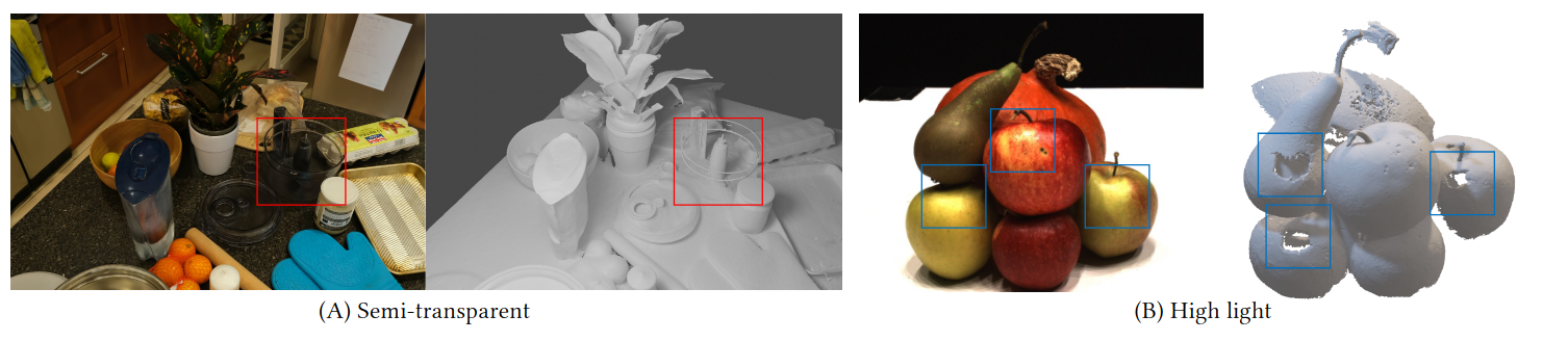
- fine geometric structure에 대해서는 덜 정확함
- regularization term사용할 때 이미지 퀄리티와 geometry간의 trade-off가 발생함 ⇒ 특정 영역에서 over-smooth결과 초래할 수 있음