Gaussian Opacity Fields, SIGGRAPH Asia 2024
Gaussian Opacity Fields: Efficient Adaptive Surface Reconstruction in Unbounded Scenes
Abstract
- 본 논문의 GOF는 ray-tracing 기반 3D Gaussian의 volume rendering을 통해 직접적으로 geometry를 추출하여 level-set을 확인하는 과정을 수행
Introduction
- NeRF 기반
- SDF(Signed Distance Function)와 occupancy 네트워크를 사용하여 surface reconstruction을 수행
- foreground object 복원에만 제한적임
- e.g., Neuralangelo
- NeRF’s opacity Field로부터 real-time rendering 및 surface 추출하는 연구도 진행됨 (e.g., Binary Opacity Grids-BOG)
- Marching Cube Algorithm
- mesh extraction Algorithm
- surface recon자체보다 NVS(novel view synthesis)에 초점이 맞춰져서 고안된 방법이라, 정규화 텀이 부족하고 다소 noisy함
- 3DGS 기반
- Poisson-Reconstruction 과 TSDF Fusion의 결함
- 포아송 재건은 Gaussian primitive에 대한 opacity(투명도), scale, rendered depth같은 정보들을 고려하지 않음
- TSDF fusion은 얇은 구조물이나 Unbounded scene에 대한 복원 성능이 정확하지 않음
Contributions
- Volume Rendering 측면 :
- projection-based 방법이랑 다르게, explicit한 ray-Gaussian intersection을 이용해서 volume rendering할 때의 Gaussian의 “기여도”를 결정함
- 이러한 ray-tracing 으로부터 기반된 formula는 ray상에 존재하는 모든 Point에 존재하는 Gaussian의 opacity를 결정짓게 할 수 있음 // (여기까진 RaDe-GS에서도 ray-tracing intersection을 이용해서 rasterized method로 가우시안의 primitive들을 풀어냈다는 점이 유사하다.)
- “view independence” = 모든 뷰에 대해 opacity가 최소인 값을 취하면 view에 대해 독립적이다(??) : opacity field가 Poisition에 대한 함수를 전적으로 책임짐
- Surface normal 측면 :
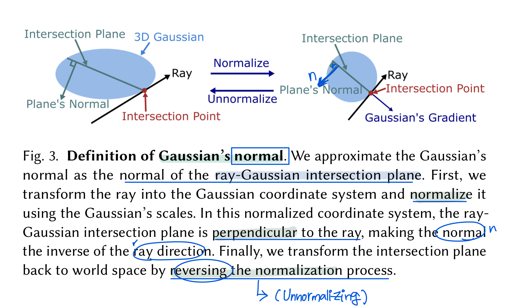
- ray와 Gausssian사이의 intersection plane(교차 평면)에 대한 normal
- Surface extraction technique(alogirthm) 측면 :
- poisson recon, marching cube와는 다른 메소드
- tetrahedra-grids(다면체 그리드)에 기반한 ‘Marching tetrahedra’ 사용함
- 3D Gaussian primitive중에서 3D bounding box의 코너값과 중앙값을 이용하여 다면체 메쉬의 꼭짓점 집합으로 구성하는 방법임
Methods
1. Modeling
- Given multiple posed + calibrated images
3D scene은 3D Gaussian의 집합 $\mathcal{G}_k$은 중심점 $\mathrm{p}_k$, scaling matrix $\mathrm{S}_k$, 그리고 rotation matrix $\mathrm{R}_k$으로 파라미터화되고, 이는 쿼터니언(quaternion, 복소수의 확장형태)로 아래처럼 나타내짐 :
\[\begin{align} \mathcal{G}_k(\mathrm{x}) = e^{-\frac{1}{2}(\mathrm{x}-\mathrm{p}_k)\Sigma_k^{-1}(\mathrm{x}-\mathrm{p}_k)} \end{align}\]
Ray Gaussian Intersection
- ray와 Gaussian이 만나는 intersection의 정도를 이용한다.
- RaDe-GS에 있던 내용이랑 겹침, 그래서 어떤 부분이 어디서부터 노벨티인지 분간이 안된다(ray tracing chapter advanced ver공부 더 해야겠다)
- “ray intersection” : 1-D Gaussian Function이 최대화되는 점
- point $\mathrm{x} = \mathrm{o} + t\mathrm{r}$ , r은 ray direction, t는 ray의 depth
local coordinate system으로 point $\mathrm{x}$ 을 변환 & scale로 normalize한다
\[\begin{align} \mathrm{o}_g &= \mathrm{S}_k^{-1}\mathrm{R}_k(\mathrm{o}-\mathrm{p}_k) \\ \mathrm{r}_g &= \mathrm{S}_k^{-1}\mathrm{R}_k\mathrm{r} \\ \mathrm{x}_g &= \mathrm{o}_g + t\mathrm{r}_g \end{align}\]ray 선 상에 존재하는 depth t에서의 1-D Gaussian value :
\[\begin{align} \mathcal{G}_k(\mathrm{t}) = e^{-\frac{1}{2}\mathrm{x}_g^T\mathrm{x}_g} = e^{-\frac{1}{2}(\mathrm{r}_g^T\mathrm{r}_gt^2 + 2\mathrm{o}_g^T\mathrm{r}_gt + \mathrm{o}_g^T\mathrm{o}_g)} \end{align}\]위의 가우시안 value가 t에 대한 quadratic term(이차형식)을 포함하고 있으므로 미분 이용해서 최대화되는 지점의 $t^*$을 유도 가능(RaDe-GS review에서 했음) :
\[\begin{align} t^* = -\frac{B}{A} \end{align}\]where, $A =\mathrm{r}_g^T\mathrm{r}_g ,$ $B = \mathrm{o}_g^T\mathrm{r}_g$
이렇게 구한 ray-Gaussian intersection은 world space에서 바로(directly) 구해질 수 있다는 점에서 surface normal구할 때도 유용한 특성임“Gaussian $\mathcal{G}_k$에 대한 기여도(Contribution) $\mathcal{E}$ 라고 정의함 :
\[\begin{align} \mathcal{E}(\mathcal{G}_k, \mathrm{o}, \mathrm{r}) = \mathcal{G}_k^{1D}(t^*) \end{align}\]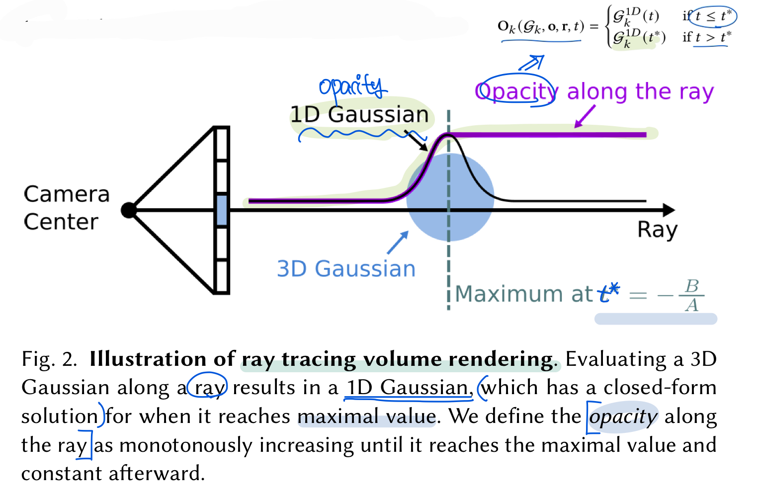
Volume Rendering
camera ray상의 pixel color는 Gaussian primitive의 depth로 정렬된 순서에 따라서 alpha blending을 통해 렌더링됨
\[\begin{align} \mathrm{c}(\mathrm{o}, \mathrm{r}) = \sum\limits_{k=1}^{K}\mathrm{c}_k\alpha_k\mathcal{E}(\mathcal{G}_k, \mathrm{o}, \mathrm{r})\prod\limits_{i=1}^{k-1}(1 - \alpha_j \mathcal{E}(\mathcal{G}_j, \mathrm{o}, \mathrm{r})) \end{align}\]
where, $c_k$ : view-dependent color modeled with spherical harmonics
and $\alpha_k$ : additional parameter that influences the opacity of Gaussian $k$.
(tile-based rendering process) 즉 standard 3DGS와 같이 depth 기반 alpha blending방식으로 pixel color rendering하는 방식 사용함
2. Gaussian Opacity Fields
projected 2D Gaussian대신 ray-Gaussian Intersection을 이용하기 때문에, ray에 존재하는 어떠한 점이라도 opacity value($\mathrm{O}_k(\mathcal{G}_k, \mathrm{o}, \mathrm{r}, t)$)를 구할 수 있다는 장점
\[\begin{align} \mathrm{O}_k(\mathcal{G}_k, \mathrm{o}, \mathrm{r}, t) = \begin{cases} \mathcal{G}_k^{1D}(t) & \text{if } t \leq t^* \\ \mathcal{G}_k^{1D}(t^*), & \text{if } t > t^* \end{cases} \end{align}\]이렇게 구해진 ray상의 opacity value를 이용하여 volume rendering process는 아래 수식처럼 이루어짐 :
\[\begin{align} \mathrm{O}(\mathrm{o}, \mathrm{r}, t) = \sum\limits_{k=1}^{K}\alpha_k \mathrm{O}_k(\mathcal{G}_k, \mathrm{o}, \mathrm{r}, t) \prod\limits_{i=1}^{k-1}(1 - \alpha_j \mathrm{O}_k(\mathcal{G}_k, \mathrm{o}, \mathrm{r}, t)) \end{align}\]이 때 3D point는 모든 뷰에서 보여지는데, 3D point $\mathrm{x}$의 opacity는 이 모든 학습 뷰에 대한 opacity value 중 최솟값으로 정의한다.
\[\begin{align} \mathrm{O(\mathrm{x})} = \min\limits_{(o, r)}\mathrm{O}(\mathrm{o}, \mathrm{r}, t) \end{align}\]위의 $\mathrm{O(\mathrm{x})}$를 "Gaussian Opacity Fields(GOF)"라고 언급한다.
- 이 GOF를 이용하면 poisson reconstruction이나 TSDF Fusion없이도 surface를 바로 추출할 수 있다.
- by identifying their level sets
- 본 논문에서 만든 Tetrahedral 기반 메쉬 추출 방법과 연결되어 사용함, 4.섹션에 더 자세히 수록
3. Optimization
- 기본적으로 2DGS에서 언급된 loss들(depth distortion, normal consistency loss)를 이용하여 정규화함
3.1. Depth Distortion loss
- Mip-NeRF360 논문에서 처음으로 제안됨
ray-Gaussian intersection들이 더 밀집되고 집중되게 해주는 것 촉진함
\[\begin{align} L_d = \sum\limits_{i,j}w_iw_j|t_i-t_j| \end{align}\]where $w_i$ : i번째 가우시안의 blending weight
\[w_i = \alpha_k\mathcal{E}(\mathcal{G}_k, \mathrm{o}, \mathrm{r})\prod_{j=1}^{k-1}(1-\alpha_j\mathcal{E}(\mathcal{G}_k, \mathrm{o}, \mathrm{r}))\]
- 하지만, depth distortion만으로는 Gaussian마다의 거리와 weight를 모두 감소시키는 정규화 텀이기 때문에, 이것은 alpha values가 증가하는 결과가 초래될 수 있다.
- alpha blending에서 섞여지는 초기 가우시안의 alpha value값이 지나치게 크다면, 과장된 Gaussian이 초래되고 이것은 "floater"를 유발하는 원인이 됨
- 따라서, 가우시안끼리의 거리에 대해서만 최소화하고, blending weight $w_i$는 최소화 텀에서 뗴어냄
3.2. Normal Consistency loss
\[\begin{align} L_n = \sum\limits_{i}w_i(1-n_i^TN) \end{align}\]- 2DGS의 normal consistency regularization을 바로 3D normal로 적용하는 것이 챌린지
- 2D Gaussian의 gradient는 항상 투영된 image plane에서의 가우시안 중심점(center, mu)에서 바깥쪽으로 위치하는 특성이 있음
- 투영된 2D 가우시안 중심에서 픽셀 좌표까지의 방향이 다르면, 두 개의 다른 픽셀에서 렌더링된 노멀은 서로 다르게 나타난다 => 정확성이 떨어지는 모호함이 발생함
이 문제 완화를 위해서 3D Gaussian의 normal을 ray direction r이 주어졌을 때, intersection plane의 normal로 정의함.
Final Loss
\[\begin{align} L = L_c + \alpha L_d + \beta L_n \end{align}\]- where, $L_c$ : RGB reconstruction loss with combining $L_1$ with the D-SSIm term
4. Surface Extraction (Marching-Tetrahedral)
- tetrahedral(다면체) 기반으로 그리드를 생성하여 메쉬 추출하는 알고리즘을 이용
- 학습 이후, surface 또는 triangle mesh extraction 단계
- 전통적인 메쉬 추출 방법들은 DTU dataset처럼 작은 물체단위의 베경없는 foreground object(regions of interest)영역은 비교적 잘 되지만, large-scale의 unbounded dataset에는 성능 좋게 나오는게 어려운 문제였음
- dense evaluation으로 하는 기존 방법 -> 그리드의 해상도에 따라 computation complexity가 증가한다는 점에서, large scale mesh에 적합하지 않고 시간이 매우 많이 걸리는 문제
- 본 논문에서 novel method 소개 : “Tetrahedral grid”를 이용한 “Marching Tetrahedra“
4.1. Tetrahedral Grids Generation
- 3D Gaussian의 primitive에서 position과 scale value는 surface의 존재에 유의미한 정보를 주는 역할
- 각각의 가우시안을 감싸는 3D Bounding box를 정의 :
- 3d box의 중심점에서 가장 높은 opacity를 가지고, 가장자리 꼭짓점(corner)에서 가장 작은 opacity를 가진다.
- 이 opacity자체를 고려하는 것은 아님, 낮은 opacity value를 가지는 가우시안을 filter out(pruning)하긴 함
- bbox의 center와 corner들로 [사면체 그리드]를 생성함
- CGAL 라이브러리 이용(Tetra-NeRF에서 영감받아 사용)해서 [Delaunay triangulation] 수행
- 들로네 삼각법이란? : 2D 평면의 점 집합을 삼각형들로 연결하는 방법 중 하나로, 삼각형의 내접원의 원 안에 다른 점이 포함되지 않도록 삼각형을 구성하는 기법
- refer : 들로네-삼각분할
- 생성된 사면체 그리드에서 filtering step을 통해 겹쳐지지 않은 가우시안과 연결된 edge를 포함하는 사면체 cell들을 제거함
- 겸쳐지지 않은 가우시안으로 판별하는 과정 : 사면체의 edge 길이가 그것에 대한 maximum scale(평균에서 3σ(표준편차)의 최대 범위까지 확장된 차원)의 합을 초과할 때
4.2. Efficient Opacity Evaluation
- 앞서 구해진 사면체 그리드의 vertices 즉, 꼭짓점에서의 opacity를 측정하기 위해, 3DGS의 rasterized method처럼 tile-based evaluation algorithm 설계함
- 꼭짓점들을 image space로 projection한 후, 타일로 쪼개져있을 때 그 대응되는 타일 ID를 확인한다.
- 각각의 타일에 대해서 projection으로 들어가져있는 point 리스트를 얻을 수 있다. 그 후에 점들을 다시 pixel space로 projection해서 대응되어 떨어지는 pixel을 구할 수 있다.
- 따라서 해당 pixel에 기여하는 가우시안들을 추적할 수 있고 이 과정은 모든 학습 이미지들에 대해서 수행된다.
- 그 후, pre-filtered된(pruning) Opcaity를 가지는 가우시안들중에서 minimum값을 Tetrahedral grid 꼭짓점의 opacity로 삼는다.
4.3. Binary Search of level Set
- traingle mesh 추출 단계 via. Marching Tetrahedral method
- “marching tetrahedral” :
- 선형 보간(linear interpolation)이 level set구분하는 것에 의존하기 때문에, Opacity Field라는 가우시안의 비선형적 특성에는 misalign되어서 성능이 불완전함
- 선형 추정(linear assumption)을 늘려가면서 non-linear한 opacity field로 level set을 정확하게 확인
- Binary Search(이진 탐색)알고리즘으로 구현함
- 8 iteration binary search한 것이 dense evaluation 256번 한 것이랑 같은 시뮬레이션 효과나오는 것 확인함

Experiments
- custom CUDA kernel
- DTU, TnT 같은 foreground simple dataset뿐만 아니라 Mip-Nerf360 dataset처럼 unbounded된 scene에서 background영역까지 복원 잘 됨
느낀점 & Future work
- ray-Gaussian Intersection(GOF)과 ray-tracing based rasterized method(RaDe-GS)에 나오는 공통 방법론이 어디서부터 시작된 이론인지 레퍼런스 찾기
- (mip-nerf 360) 논문에서 depth distortion loss 부분 중심으로 읽기 (완)
- 들로네 삼각분할 « 대충 훑기만 해선 이해안됨
- 포아송 재건, 마칭큐브// 마칭-사면체 같은 메쉬추출 알고리즘만 정리돼있는 내용 어디없는지 확인