RaDe-GS, arXiv preprint
RaDe-GS: Rasterizing Depth in Gaussian Splatting
Abstract
- 3DGS의 이산적이고 비구조적인 특성때문에 shape accurac가 떨어지는 문제 있음
- 최근 관련 연구 중, 2D-GS에서는 shape reconstruction 성능을 올리기 위해, Gaussian primitives들을 이용했지만 이것은 렌더링 퀄리티랑 계산적인 효율성은 감소시키는 효과가 있음
- 그래서 본 논문에서는 rasterized 접근법을 통해, 3DGS의 depth map과 surface normal map을 렌더링하는 Shape reconstruction 정확성 보장
- DTU dataset에서 NeuraLangelo와 비교했을 때 CD(Chamfer Distance) error가 좋게 나옴
Introduction
- multi-view 이미지들로부터 3D Reconstruction하는 태스크에서는 multi-view stereo 알고리즘을 통해 depth map을 얻는 것을 포함한다.
- 이렇게 얻어진 depth map으로 완전한 triangle mesh를 만드는 모델로 통합되는 것이 가능하다
전통적인 image-based 모델링 접근법은 꽤 정확한 결과로 depth map rendering + mesh recon이 가능하나, 고질적으로 빛나는 표면(shiny surface)이나 reflective한 유리같은 transparent surface에서 특히나 robustness가 떨어지는 한계점이 존재한다.
- explicit한 3DGS에서 surface 잘 뽑아내는 것은 어려운 문제임
- 2DGS[Huang et al.2024] : PSNR 수치 줄어듦
- GOF[Yu et al.2024] : ray-tracing 기반 방법을 통해 광선(light ray)에 따른 Gaussian opacity를 계산하는 방법으로 high-quality surface를 뽑아냄
Contributions
- 본 논문에서는 raasterized 기반 방법으로 general Gaussian Splatting에서 정확한 depth map을 얻는 것을 발전시켰다.
- standard GS만큼의 computation efficiency를 가진다.
- DTU dataset에서 shape reconstruction accuracy를 Chamfer Distance 0.69mm 달성, 5분의 학습시간
- 이 수치는 implicit한 representation 기반 모델인 NeuraLangelo(0.69mm)와 비슷
- GS-based 방법론들(sota는 GOF)에서는 당연히 성능 더 좋았음
Methods
- scene에 splatting된 Gaussian들과 광선에 의한 intersection point를 통한 솔루션을 찾음
> camera center로부터 각각의 Light ray에 의해 Gaussian value가 최대화되는 지점이 intersection point이다
> intersection point들에서 Affine-projection을 시키면 co-planar (동일 평면상에 존재)하다
> 그리고 이 intersection point들을 Image plane에 projection 된 depth로 정의하여 curved surface를 구할 수 있다
> 따라서, planar equation으로 projected depth를 구하는데 이것은 rasterization에 의해 효율적으로 계산될 수 있다.
> final depth map은 투명도(translucency)를 고려하여 투영된 Gaussian들 중에서 중간값 깊이(median depth)로 계산
1. Rasterizing Depth for Gaussian Splats
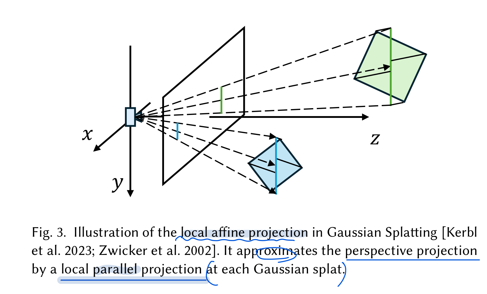
Gaussian Splatting에서는 아래 사진처럼 Perspective camera projection을 Affine transformation을 통해 근사시켜서 더 효율적인 rendering가능하다는 것 사전에 알아두고 시작
- standard 3DGS에서는 알파 블렌딩을 위해서 image plane에 projected된 2D Gaussian의 중심점(center)을 depth로 설정한다.
- shape detail 포착 불가능
- 그러므로, 본 논문에서는 spatially varying depth를 rasterized method기반 방법으로 계산한다.
1.1. Depth Under Perspective Projection
- planar equation을 얻는 본격적인 과정 이전에, perspective projection으로 camera coordinate에 대한 기본 concepts부터 먼저 이해해보자.
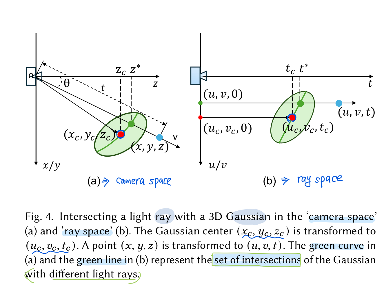
- Figure 4.
- Figure 4.
위 그림에서 왼쪽의 (a)에서 보여진 것 처럼, camera center $\mathrm{o}$와 unit direction $\mathrm{v}$가 주어졌을 때,
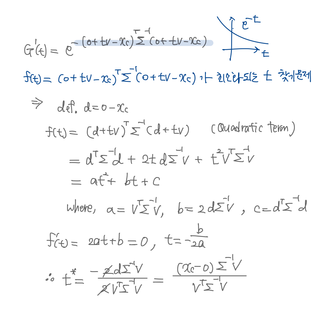
ray 상에 $o$로부터 거리 $t$만큼 떨어져 있는 point $\mathrm{x}$는, \(\begin{align} \mathrm{x}= \mathrm{o} + t\mathrm{v} \end{align}\) 으로 구할 수 있다.이 ray에 존재하는 Gaussian value $\mathrm{G}^1(t)$는, \(\begin{align} \mathrm{G}^1(t)= e^{-(\mathrm{o} + t\mathrm{v}-\mathrm{x}_c)^T\Sigma^{-1}(\mathrm{o} + t\mathrm{v}-\mathrm{x}_c)} \end{align}\) 으로 구할 수 있다.
- 이 때, Gaussian value는 1-D function이고, 이 값이 최대화되는 지점이 3D Gaussian과 ray가 만나는 “intersection point” 라고 정의한다.
그 후 distance $t^*$ : intersection point와 camera center간의 거리는 위의 Gaussian value가 최대화되는 t를 찾으면 되고 구한 식은 아래처럼 됨
\[\begin{align} t^* = \frac{\mathrm{v}^T\Sigma^{-1}(\mathrm{x}_c - \mathrm{o})}{\mathrm{v}^T\Sigma^{-1}\mathrm{v}} \end{align}\](유도 과정) :
- 이렇게 유도된 distance $t^*$이 의미하는 바는, 3D Gaussian들과 광선들 집합간의 intersection들이 “curved surface”(연두색 곡선) 를 나타낸다고 해석할 수 있음
- different pixels have different depth values of $t^*$ and different viewing direction $\mathrm{v}$.
1.2. Depth Under Local Affine Projection
- 이제 가우시안말고, 픽셀의 depth를 “local affine projection”으로 구해보자.
위의 Figure4.(b)상황 => “ray space” 좌표계
[1.2.1. Transformation from Camera to Ray space]
- (a) 의 파란 점 $\mathrm{x} = (x, y, z)^T$ 가 (b)의 파란 점 $\mathrm{u} = (u,v,t)$ 로 변환
- $(u,v,t)$에서 $(u,v)$는 image plane coordinate(이미지 평면에서의 좌표계)이고, $(t)$는 point와 $uv-plane$사이의 거리를 나타낸다
- 즉, $t=\sqrt{x^2+y^2+z^2}$
ray space에서 light direction $\mathrm{v}$ 는 단위고유벡터 $(0,0,1)^T$임
가우시안들도 ray space로 변환되어야 하는데, 변환된 Gaussian Function은 아래와 같다
\[\begin{align} \mathrm{G}'(\mathrm{u}) = e^{-(\mathrm{u}-\mathrm{u_c})^T\Sigma^{'-1}(\mathrm{u}-\mathrm{u_c})} \end{align}\]Gaussian center $\mathrm{u_c}=(u_c, v_c, t_c)^T$로, (b)그림에서 빨간 점
[1.2.2. Intersection in Ray Space]
기본 과정은 perpective projection때와 같음
1) ray space 상에 존재하는 point $\mathrm{u}$ :
\[\begin{align} \mathrm{u} = \mathrm{u_o} + t\mathrm{v'} \end{align}\]where , $\mathrm{u_o} = (u,v,0)^T \quad and \quad \mathrm{v’} = (0,0,1)^T $
2) 1D Gaussian function $\mathrm{G^{‘1}}(t)$ :
\[\begin{align} \mathrm{G^{'1}}(t)= e^{-(\mathrm{u_o} + t\mathrm{v'}-\mathrm{u_c})^T\Sigma^{'-1}(\mathrm{u_o} + t\mathrm{v'}-\mathrm{u_c})} \end{align}\]3) maximum point가 위치한 distance $t^*$ :
\[\begin{align} t^* = \frac{\mathrm{v'}^T\Sigma^{'-1}(\mathrm{u}_c - \mathrm{u_o})}{\mathrm{v'}^T\Sigma^{'-1}\mathrm{v'}} \end{align}\]간단하게 표현하기 위해서 $(\mathrm{u}_c - \mathrm{u_o})$ 벡터 빼고 나머지 항들을 $\hat{q}$로 정의하여 간단하게 아래처럼 표현 :
\[\begin{align} t^* = \hat{q}(\mathrm{u}_c - \mathrm{u_o}) \end{align}\][1.2.3. Depth of Intersection]
1) $t$는 3D point $x$와 camera center $o$사이의 거리이므로 x에 대한 깊이는, 간단하게 삼각비 성질을 이용해서 (a)그림의 $z^*$을 아래처럼 구할 수 있다:
\[\begin{align} d = cos\theta t^* \end{align}\]2) (b), affine projection인 상황에 대입해서 depth구하면,
\[\begin{align} d = cos\theta_c t^* = \frac{x_c}{t_c}t^* = \frac{x_c}{t_c}\hat{q}(\mathrm{u}_c - \mathrm{u_o}) = \hat{p}(\mathrm{u}_c - \mathrm{u_o}) \end{align}\]여기서 $\hat{p} = \frac{z_c}{t_c}\hat{q}$로 정의
3) 이어서 위의 식을 아래처럼 나타낼 수 있는데,
\[\begin{align} d = \hat{p}(\mathrm{u}_c - \mathrm{u_o}) = \hat{p}\begin{pmatrix} u_c - u \\ v_c-v \\ t_c \end{pmatrix} = \hat{p}\begin{pmatrix} 0 \\ 0 \\ t_c \end{pmatrix} + \hat{p}\begin{pmatrix} \Delta{u} \\ \Delta{v} \\ 0 \end{pmatrix}. \end{align}\]4) 위의 최종 분해된 식 중, 첫 번째 항 $\begin{pmatrix} 0 \ 0 \ t_c \end{pmatrix}$에 대한 성질 :
\[\begin{align} \hat{p} \begin{pmatrix} 0 \\ 0 \\ t_c \end{pmatrix} &= \frac{z_c}{t_c} \hat{q} \begin{pmatrix} 0 \\ 0 \\ t_c \end{pmatrix} \\ &= \frac{z_c}{t_c} \frac{\mathrm{v^{'T}}\Sigma^{'-1}}{\mathrm{v^{'T}}\Sigma^{'-1}\mathrm{v'}} \begin{pmatrix} 0 \\ 0 \\ t_c \end{pmatrix} \\ &= \frac{z_c}{t_c} \frac{\mathrm{v^{'T}}\Sigma^{'-1}}{\mathrm{v^{'T}}\Sigma^{'-1}\mathrm{v'}} (t_c\mathrm{v'}) \\ &= \frac{z_c}{t_c} \frac{\mathrm{v^{'T}}\Sigma^{'-1}\mathrm{v'}}{\mathrm{v^{'T}}\Sigma^{'-1}\mathrm{v'}} (t_c) \\ &= z_c . \end{align}\]
5) 두 번째 항의 $\hat{p}$ 는 $p$ 로 근사됨- 따라서, 최종적으로 depth를 구하는 rasterized method수식으로 유도된다.
- Recall. $d = z_c + p(\begin{pmatrix} \Delta{u} \ \Delta{v} \end{pmatrix})^T$
2. Rasterizing Normal for Gaussian Splats
느낀점
- 이 분야에서는 살짝 뭐 바꿨더니 소타다 이런건 절대 안먹히겠다
- 완전히까진 아니여도 적당히 창의적으로 메소드를 짜야되겠구나라는 생각이 들었다. 이런 면이 재밌지만서도 다소 막막하긴 하다
- Affine aprroximation projection기반으로 spatial varying depth 구하는 방법이 창의적이다
- 2DGS에서 쓴 loss 가져다 쓴 건 아쉬운데 이거까지 새로 짰으면 걍 씨그라프 오랄 찍었을 것 같다
- 이건 어셉 왜 안되지
- GOF(SIGGRAPH Asia 2024)가 작년 9월에 나와서 sota인 것 같다. 이어서 이거 읽기