Graphics-Ch4. Ray Tracing

Rendering

1. Object based Rendering
   • 각각의 object단위로 고려됨
   • 물체가 존재하는 모든 픽셀들이 찾아지고 업데이트 됨
2. Image based Rendering
   • 각각의 pixel단위로 고려됨
   • 물체에 영향을 주는 각 pixel들이 찾아지고 업데이트 됨
     둘의 차이점에 대해서는 ch8에서 더 자세하게 다룬다

Ray Tracing이란

• 3D Scene을 렌더링하는데에 사용되는 image-order 알고리즘
• object-order rendering에서 사용되어지는 수학적 방법

1. Basic Ray-Tracing Algorithm

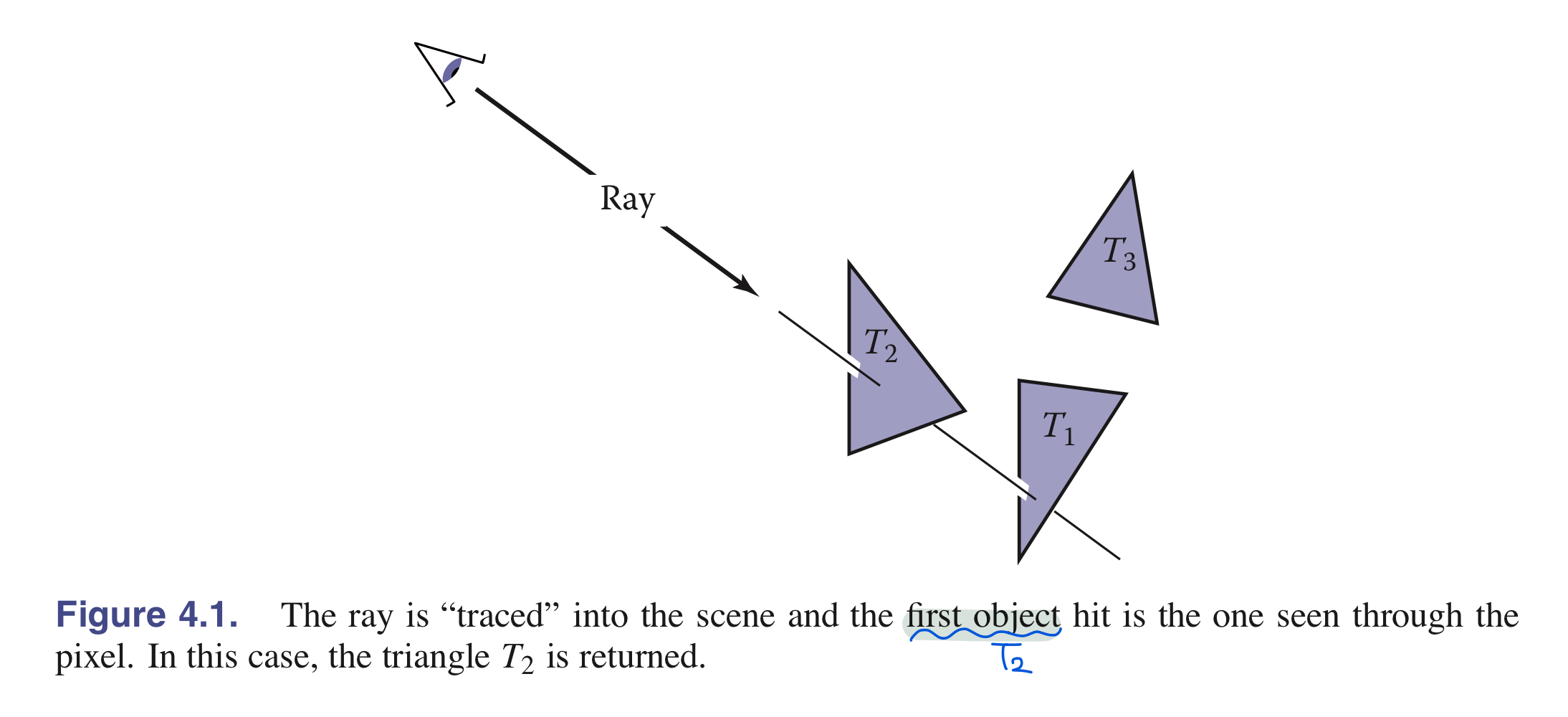
• image상의 Pixel에서 ray tracing을 했을 때 보여지는 물체를 찾는 것이 목표
• 각각의 픽셀은 다른 방향을 “바라본다”
  • 이 보여지는 물체들은 모두 viewing ray 상에 존재한다
• 카메라에 가장 가깝게 존재하는 viewing ray에 대해 교차하고 있는 특정 Object를 찾는 것이 목표

• 그 물체가 찾아지면, shading 계산을 통해 intersection point, surface normal, 그리고 다른 정보들을 구해서 pixel color를 결정할 수 있음

• Basic Ray Tracer의 세 가지 흐름 :
  1. Ray Generation : Camera geometry에 기반하여, origin과 각 픽셀마다 vieweing ray의 direction을 구하는 것
  2. Ray Intersection : viewing ray와 교차하는 가장 가까운 물체(Object)를 찾는 것
  3. Shading : ray-intersection 과정을 통해 구해진 결과를 기반으로 Pixel color를 계산하는 것
• 기본 내용을 다룬다, 더 발전된 내용은 chapter 10, 12, 13 등등에 나옴
  

2. Perspective projection

• how to mapping 3D objects into 2D image plane?

  1. Linear perspecrive

     straight line => straight line

  2. Parallel projection

     projection direction에 따라서 움직여짐

     • parallel projection을 통해 보이는 뷰는 orthographic view라고도 부른다
     • 장점 : 변환되어도 size랑 shape은 변화시키지 않고 일정하게 유지한다
     • 단점 : 물체가 view point기준으로 멀어질수록 작게 보인다 => vanishing point(소실점)과 연관 있음
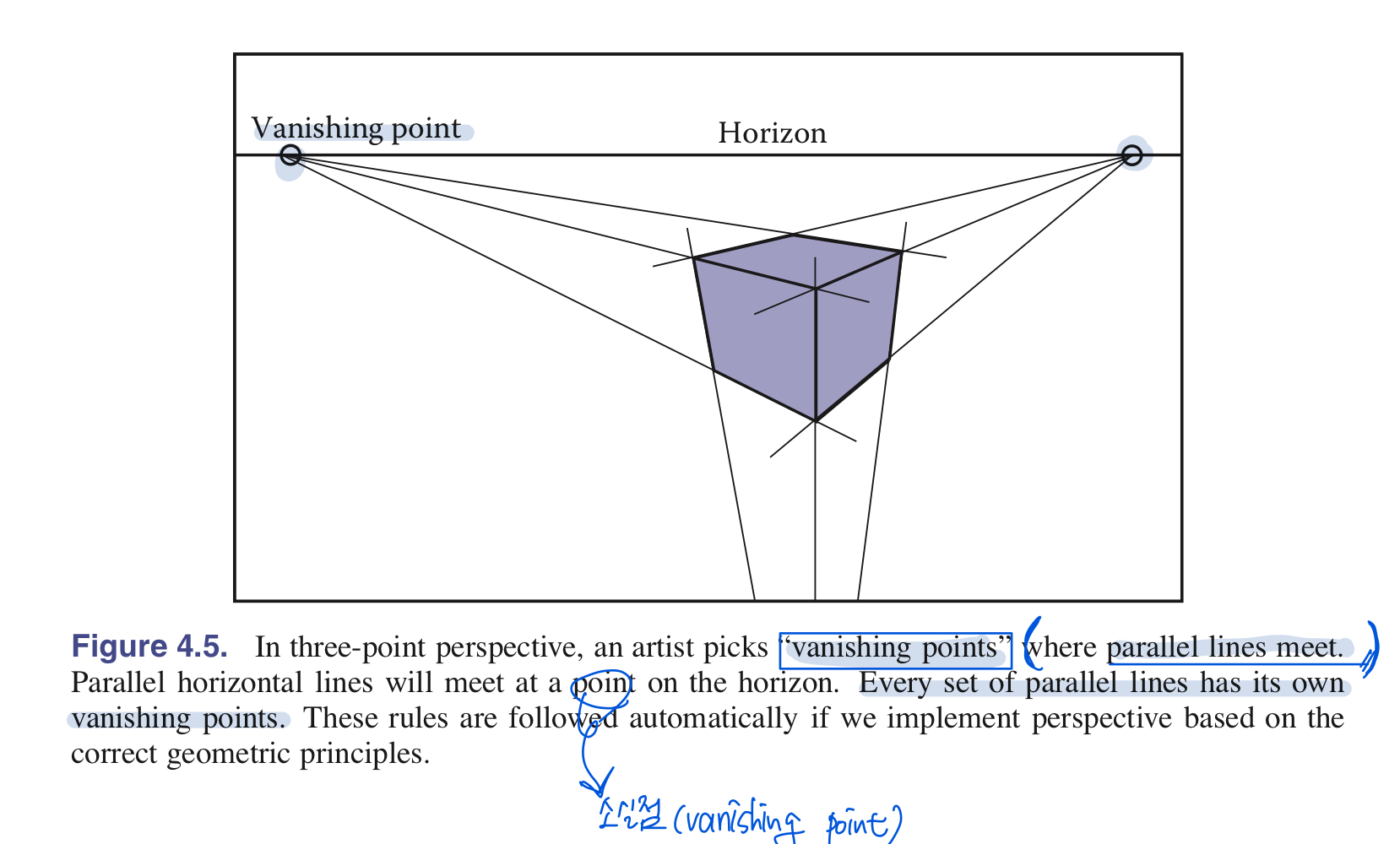
       • this is because eyes and cameras don’t collect light from a single viewing direction(뷰 하나 보이는 것으로 눈과 카메라에서 모든 빛을 수집할 수 없기 때문임)
         

3. Computing Viewing Rays (Ray Generation)

\(p(t) = e + t(s-e)\)

• $e$ : eye(origin point, view point)
• $s$ : end point of the ray

• $t$ : 시간 축
  

• vector $(s-e)$ 를 view direction로 해석할 수 있다
• 만일 $t$가 0보다 작다면, view behind에 있다고 해석할 수 있다
• “Ray Generation” 단계의 origin과 view direction을 구하는 과정에서 camera frame으로 알려진 orthonormal 좌표계에서 시작해야 한다.
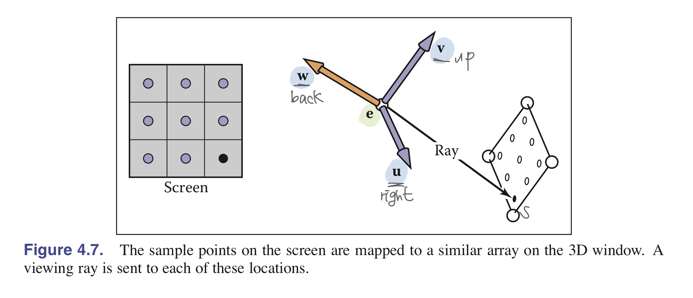
  • orthonormal coordinate frame : 세 가지 기저 벡터 $u, v, w$으로 구성되어 있음

3.1. Orthographic (Parallel) Views

• 이미지를 표현하는 4가지 차원 = ${l, r, b, t}$
  

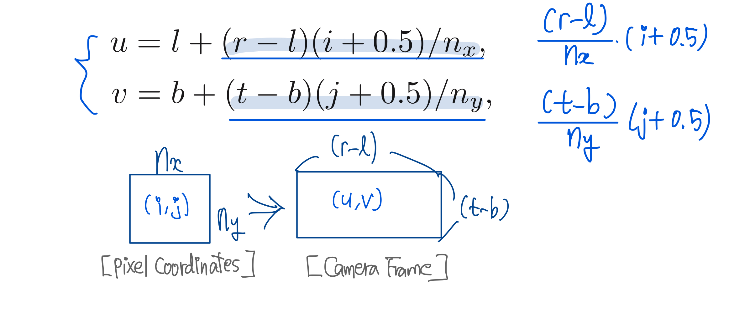
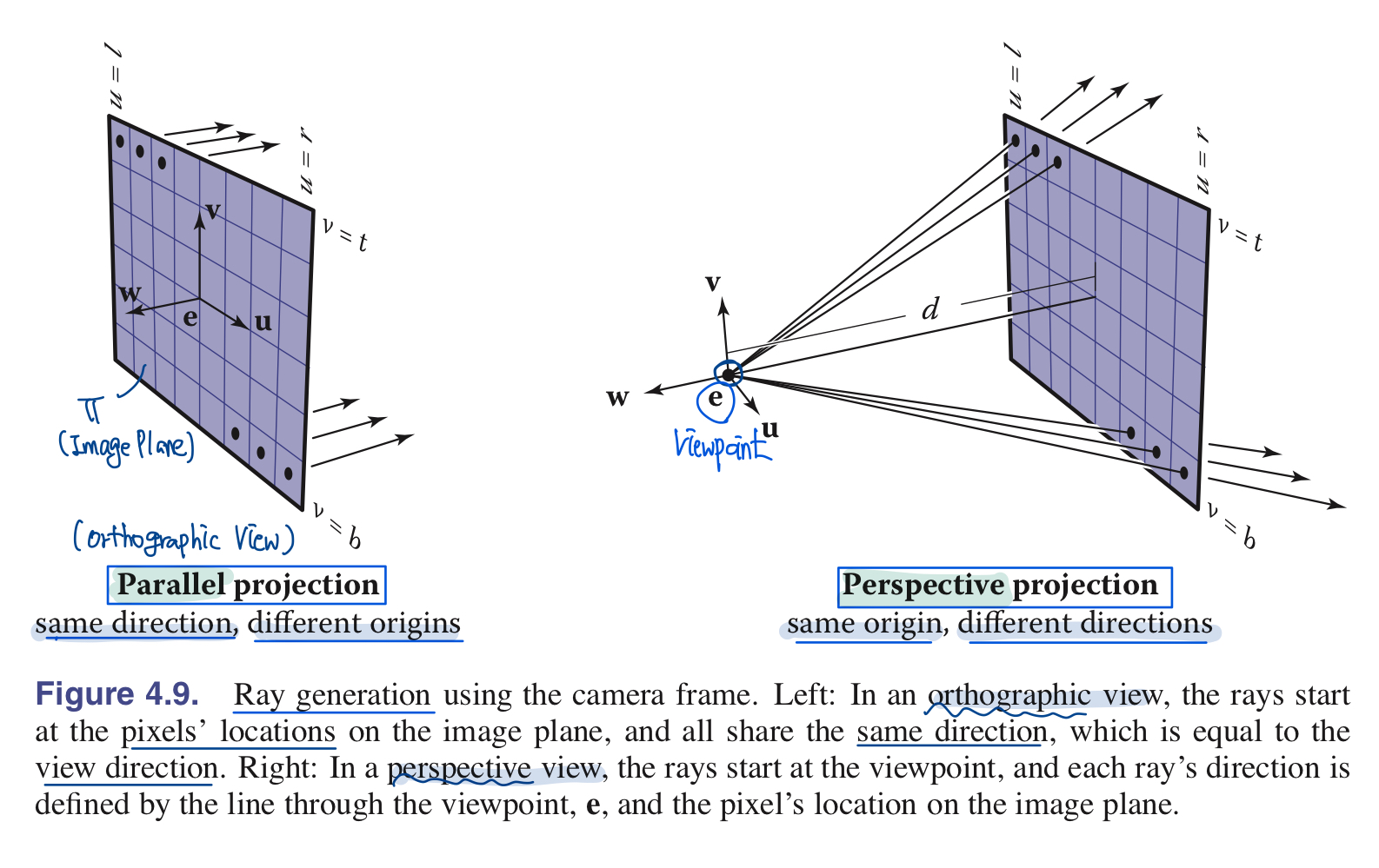
[Orthographic viewing rays 만드는 방법]

• ray Starting point(Origin)로 pixel의 image-plane position을 그대로 사용할 수 있다 = $e + u\mathrm{u} + v\mathrm{v}$
• ray’s Direction으로는 view direction을 가져다가 사용할 수 있다 = $-w$

3.2. Perspective Views

• 각 픽셀마다의 ray들은 같은 origin$(e)$를 공유함
  • Image Plane이 더이상 $e$ 점에 위치하는 것이 아니라, 거리 $d$만큼 떨어져서 존재함
  • $d$ : image plane distance 또는 focal length 라고 불린다
• view direction은 모두 다름
  • 어떻게 구해지는가? -> image planedml pixel위치와 viewpoint에 의해서 정의된다 = $-dw + u\mathrm{u} + v\mathrm{v}$

4. Ray-Object Intersection

• 앞선 Ray Generation단계를 통해 ray $\mathrm{e} + t\mathrm{d}$를 만들었다면,
  $t > 0$ 인 구간에서 ray와 처음으로 교차되는(만나는) 물체를 찾는 것이 필요하다.
• General problem = find the first intersection between the ray & a surface that occurs at a $t$ in the interval $[t_0, t_1]$
  • sphere과 traingles 물체(surface)를 먼저 다루고, 다른 다면체들은 다음 섹션에 다루겠음

4.1. Ray-Sphere Intersection

다음의 ray와 surface가 만나는 교차점을 구한다고 생각해봅시다,

• ray $p(t) = \mathrm{e} + t\mathrm{d}$
• implicit surface $f(p) = 0$

\[\begin{align} f(p(t)) = 0 \\ f(\mathrm{e} + t\mathrm{d}) = 0 \end{align}\]

• 그리고 sphere는 중심점 $c = (x_c, y_c, z_c)$와 반지름 $R$을 이용해서 아래처럼 implicit equation을 나타낼 수 있음 \(\begin{align} (x - x_c)^2 + (y - y_c)^2 + (z - z_c)^2 - R^2 = 0 \\ (p-c) \cdot (p-c) - R^2 = 0 \end{align}\)

• 이 vector form 구의 방정식에서 p에다가 ray $p(t)$를 집어넣어도 식이 성립해야 함, intersection point이기 때문

  $(\mathrm{e} + t\mathrm{d} - c) \cdot (\mathrm{e} + t\mathrm{d} - c) - R^2 = 0$

• 식을 풀면 아래와 같이 $t$에 대한 2차방정식 term으로 풀어짐

  $(d \cdot d)t^2 + 2d \cdot (e-c)t + (e-c) \cdot (e-c) - R^2 = 0$

• 근의 공식을 이용하여 $t$를 구한다 \(t = \frac{-d \cdot (e-c) \pm \sqrt{(d \cdot (e-c))^2 - (d \cdot d)( (e-c) \cdot (e-c) - R^2)}}{(d \cdot d)}\)

• 근의 공식 풀기 위해서는 판별식 ($B^2 - 4AC$) 이거를 통해 근이 몇 개 나오는지 먼저 판단한다, 이 값이 음수면 허수라서 교차점 없다고 판단하면 됨

• section 2.5.4에서 다루었던 것처럼, point $p$에 있는 normal vector는 gradient를 통해 아래처럼 계산할 수 있음

  \mathrm{n} = 2(p-c)

• unit normal = (p-c) / R

4.2. Ray-Traingle Intersection

• barycentric 좌표계 사용함
  => 삼각형을 포함하는 parametric plane을 표현할 때 삼각형의 꼭짓점만 이용하면 다른 storage가 필요없는 효율적인 좌표계표현이기 때문
  
• parameteric surface와 ray간의 intersection point구하는 방법 :
  • Cartesian coordinate (데카르트 좌표계)를 이용한 다음 연립방정식으로 푼다 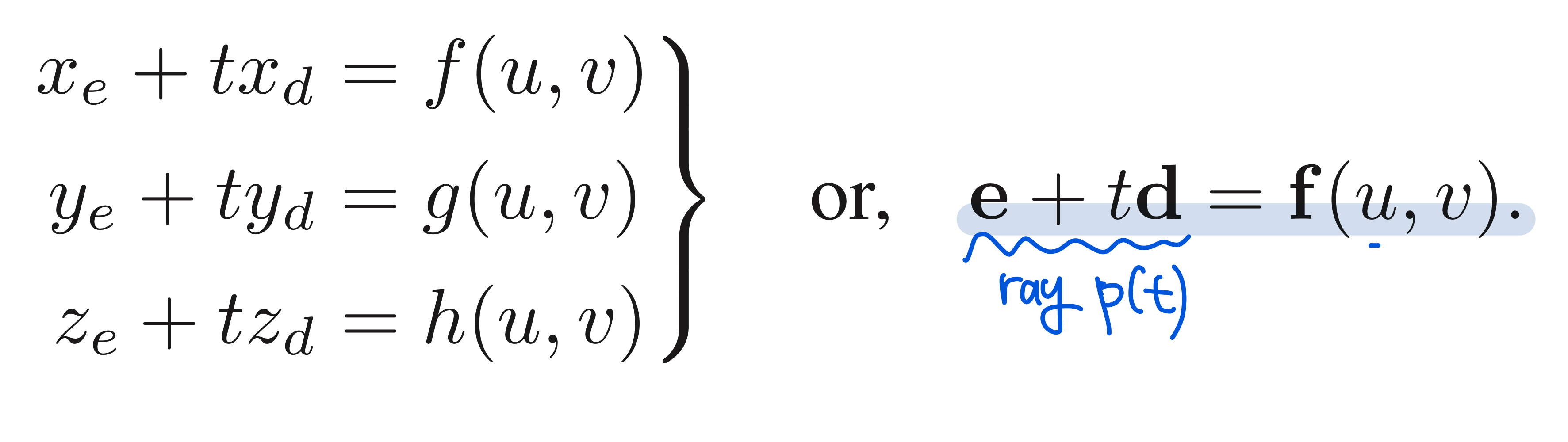=> 식이 세 개이고, 구해야 되는 미지수도 $(t, u, v)$로 세 개이기 때문에 계산 가능

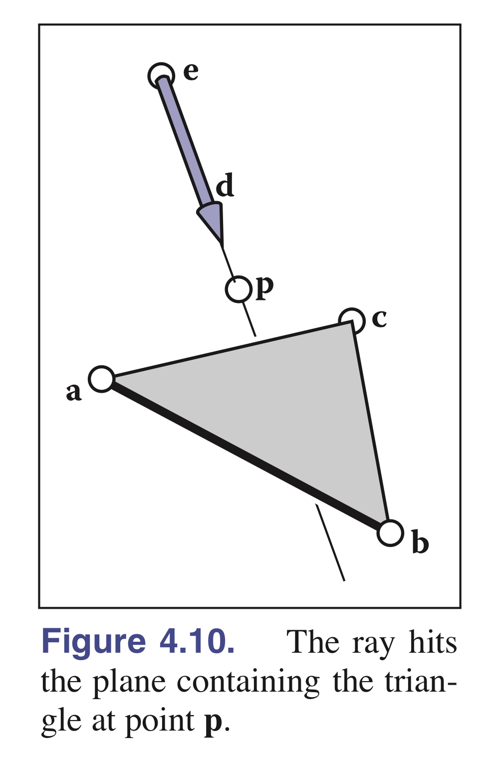왼쪽 그림과 같이, $a,b,c$ 의 vertices로 이루어진 삼각형이 존재하고 ray $p(t) = \mathrm{e} + t\mathrm{d}$가 존재하는 상황을 가정할 때, intersection point인 $p$는 그림과 같이 ray 연장선 위에 존재한다. $$ \mathrm{e} + t\mathrm{d} = \mathrm{a} + \beta(\mathrm{b} - \mathrm{a}) + \gamma(\mathrm{c}-\mathrm{a}) $$ 이 식에서 $t, \beta, \gamma$를 구해야 함

위의 식을 vector form으로 아래처럼 식을 확장할 수 있음 :

\[\begin{align} x_e + tx_d = x_a + \beta(x_b - x_a) + \gamma(x_c - x_a), \\ y_e + ty_d = y_a + \beta(y_b - y_a) + \gamma(y_c - y_a), \\ z_e + tz_d = z_a + \beta(z_b - z_a) + \gamma(z_c - z_a). \\ \end{align}\]

• vector form을 행렬로 바궈서 standard linear system(선형 결합 형태)로 아래처럼 바꿔 표현 가능:

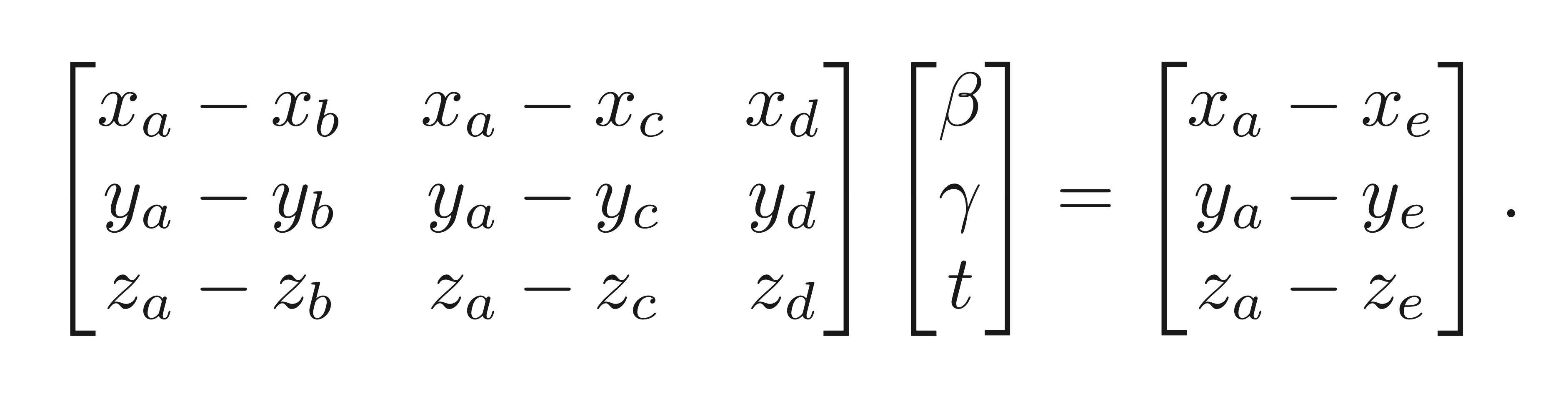
• 그 후, 크래머 규칙(Cramer’s rule)을 이용해서 $t, \beta, \gamma$ 값을 도출할 수 있다 (자세한 풀이 생략 책 참고)

5. Shading

• 픽셀에 대한 intersection point, 즉 visible surface가 구해졌다면, 광원을 고려해서 pixel color(intensity) 결정하는 단계
• Light Reflection(반사) 관련 모델링을 사용한다
  • 중요한 변수들
    1. light direction $\mathrm{l}$
    2. view direction $\mathrm{v}$
    3. surface normal $\mathrm{n}$

5.1. Lambertian Shading

• 가장 간단한 shading modeling 을 위한 가정

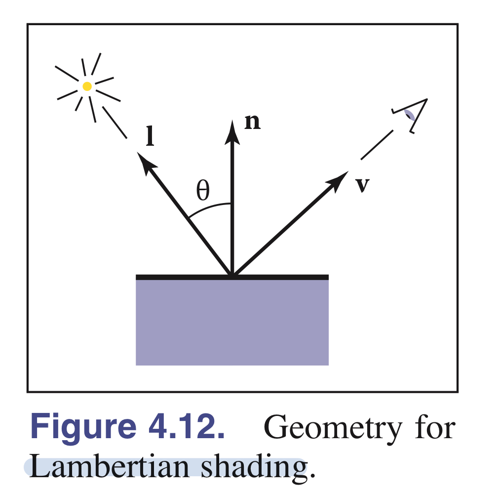**Lambertian Shading** : 왼쪽 그림에서 표면에 떨어지는 광원으로부터 나오는 빛의 양은 빛에 대한 입사각 $\theta$에 의해서만 결정된다. (View-Independent) 이를 이용해서 lambertian Shading model식을 아래처럼 설계 $$ L = k_d I max(0, \mathrm{n} \cdot \mathrm{l}) $$

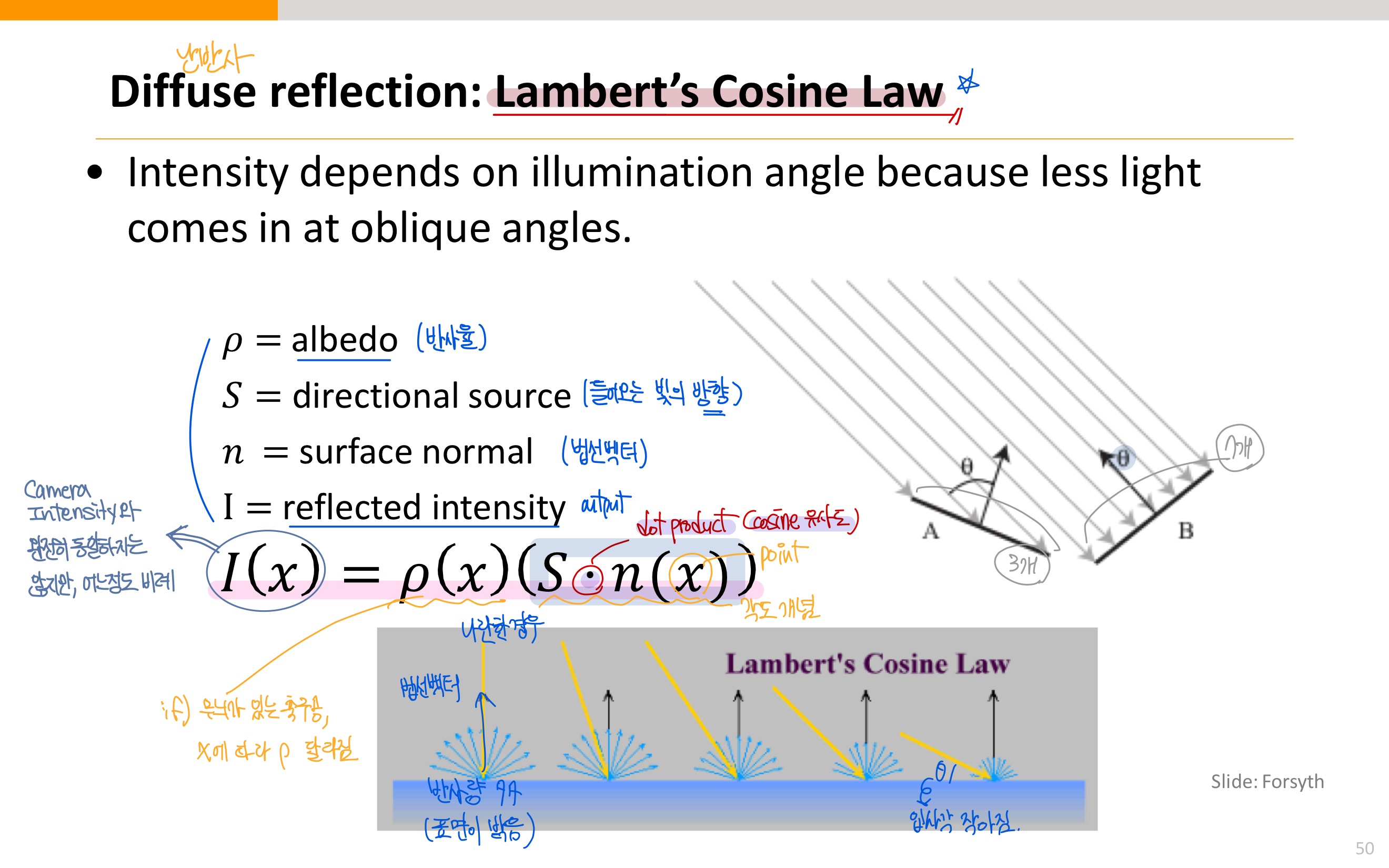
• $k_d$ : diffuse coefficient (난반사 계수) 또는 surface color = 표면이 입사된 빛을 얼마나 균일하게(난반사로) 반사하는지를 나타내는 계수
• $I$ : intensity of the light source
• 여기서 n과 l은 크기가 1인 단위벡터이기 때문에, $\mathrm{n} \cdot \mathrm{l}$을 $cos\theta$ 로 계산 가능하다.
  • 즉, 내적은 cosine 유사도를 의미하므로 빛이 들어오는 방향에 대해서 얼마나 반사되는지 그 강도(intensity)가 결정된다는 의미

=> 위의 모델링 수식은 RGB 채널 3개에 대해서 각각 적용되어 pixel value가 구해진다

• $\mathrm{v}, \mathrm{l}, \mathrm{n}$이 모두 단위벡터(크기가 1)인 것을 잊지 말기!

5.2. Blinn-Phong Shading

• 모든 광원이 난반사(diffuse)로만 구성되지는 않는다,
• specular component (정반사되는 성질) 빛을 모델링하기 위한 모델
• Idea : $\mathrm{v}$랑 $\mathrm{l}$ 이 surface normal $\mathrm{n}$을 가로지르는 상황에서 반사가 가장 잘된다는 것
  • mirror reflection이 발생할때 반사율이 가장 크다.

오른쪽 그림처럼, $\mathrm{v}$와 $\mathrm{l}$ 각도 중간에 위치한 half vector $\mathrm{h}$가 있다고 가정해보자, 이 h가 surface noraml n과 가까울수록, specular component가 증가한다. (밝기가 증가) $\mathrm{h}$와 $\mathrm{n}$사이의 유사도는 **dot product(내적)**으로 생각할 수 있다. *Phong exponent*라고 불리는 power $p$가 surface에 대한 광택의 정도를 조절하는 역할임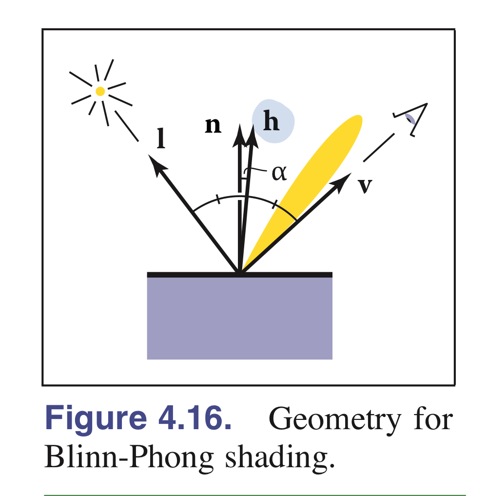

\[\begin{align} h = \frac{\mathrm{v} + \mathrm{l}}{||\mathrm{v} + \mathrm{l}||}, \\ L = k_d I max(0, \mathrm{n} \cdot \mathrm{l}) + k_s I max(0, \mathrm{n} \cdot \mathrm{h})^p \\ \end{align}\]

where, $k_s$ is the specular coefficient, or the specular color of the surface

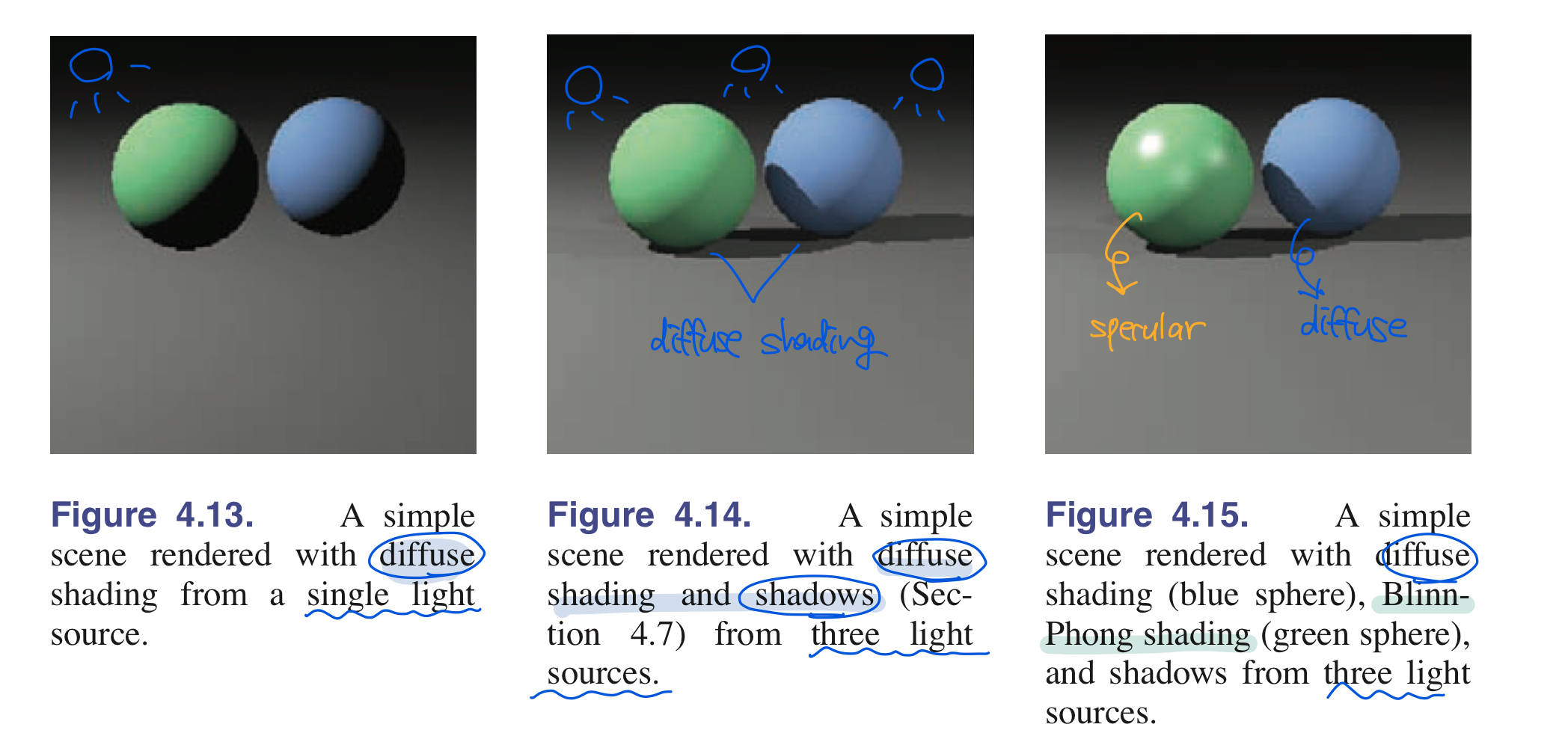
5.3. Ambient Shading

• 조명이 도달하지 않는 표면에서는 완전하게 black으로 보이기 때문에, 이런 현상을 줄이기 위해서 constant component를 shading model에 추가시킴

• Full version of a simple and useful shading model(Ambident shading components & Blinn-Phong model) :

  \[\begin{align} l = k_aI_a + k_dImax(0, \mathrm{n} \cdot \mathrm{l}) + k_s I Max(0, \mathrm{n} \cdot \mathrm{h})^n\\ \end{align}\]