Graphics-Ch6. Transformation Matrices

Introduction

• Chapter 5는 선형대수학(Linear Algebra)이라 아는 내용이 많아서 정리 생략
• Transformation matrix는 왜 필요한가 : Rotation, Translation, Scaling, Projection같은 기하학적 변환에서 행렬 곱을 통해 변환되는데 이때 변환 행렬이 필요함

1. 2D Linear Transformations

• 2D vector를 2x2 행렬로 변환하는 과정은 아래처럼 전개됨 :
  

  \[\begin{bmatrix} a_{11} & a_{12} \\ a_{21} & a_{22} \end{bmatrix} \begin{bmatrix} x \\ y \end{bmatrix} = \begin{bmatrix} a_{11}x & a_{12}y \\ a_{21}x & a_{22}y \end{bmatrix}\]

• 여기서, 벡터 $(x y)^T$에 곱해지는 행렬 $A$를 변환행렬이라고 한다

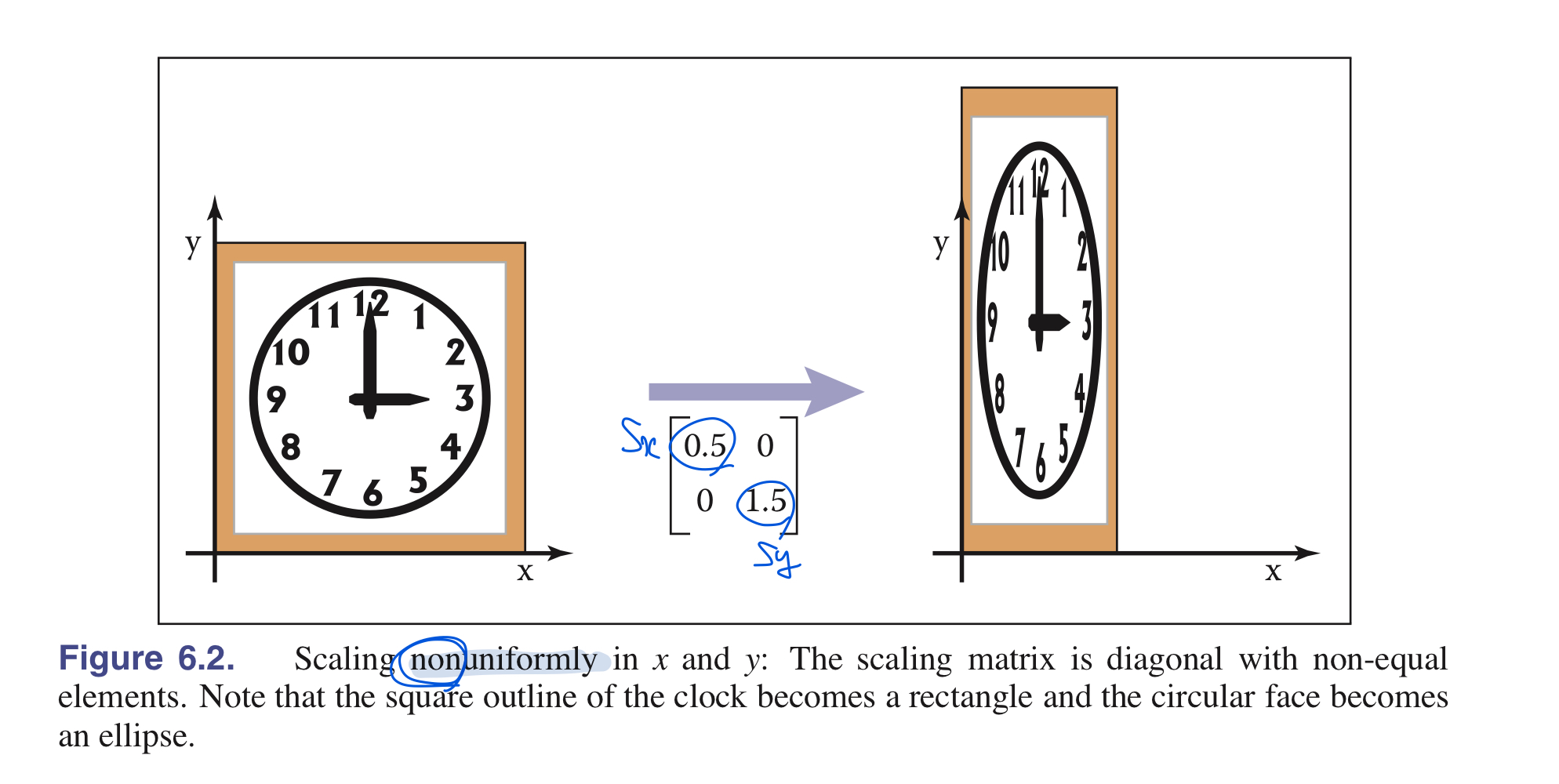
1.1. 2D Scaling

\[\begin{align} scale(s_x, s_y) = \begin{bmatrix} s_x & 0 \\ 0 & s_y \end{bmatrix} \end{align}\]

=> Cartesian components와 결합되면 아래와 같이 전개됨

\[\begin{bmatrix} s_x & 0 \\ 0 & s_y \end{bmatrix} \begin{bmatrix} x \\ y\end{bmatrix} = \begin{bmatrix} s_xx \\ s_yy \end{bmatrix}\]

1.2. Shearing

• 물체에 평행한 방향으로 힘이 가해져 변형되는 현상

• 얼만큼($=s$만큼) x또는 y방향으로 물체를 밀 건지

  \[shear-x(s) = \begin{bmatrix} 1 & s \\ 0 & 1 \end{bmatrix} , shear-y(s) = \begin{bmatrix} 1 & 0 \\ s & 1 \end{bmatrix}\]

• 만약, 시계 방향으로 각도 $\phi$만큼 회전시키는 shear transformation matrix : \(\begin{bmatrix} 1 & tan\phi \\ 0 & 1 \end{bmatrix}\)

• 만약, 반시계 방향으로 각도 $\phi$만큼 회전시키는 shear transformation matrix : \(\begin{bmatrix} 1 & 0 \\ tan\phi & 1 \end{bmatrix}\)

1.3. Rotation

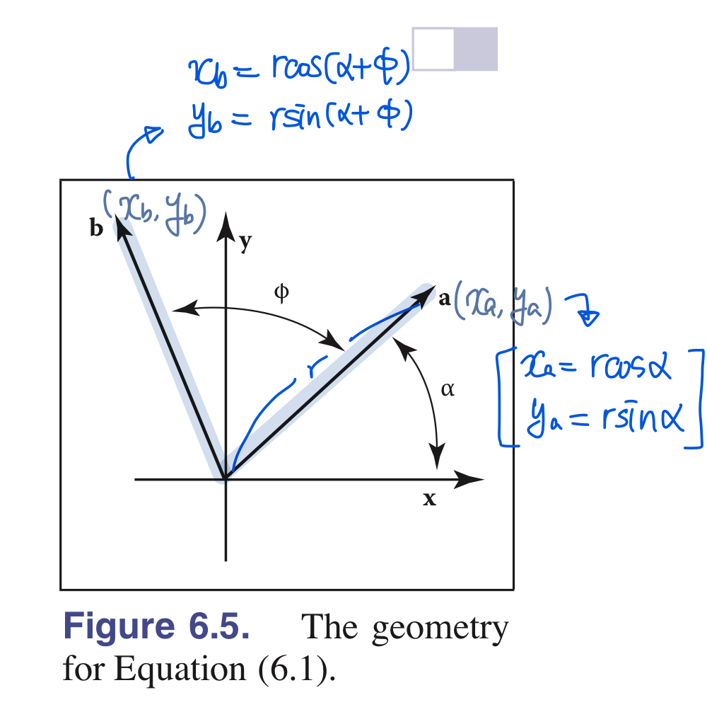vector $\mathrm{a}$가 x축으로부터 각도 $\alpha$만큼 떨어진 길이가 r인 벡터라는 상황 가정 반시계방향(counterclockwise)으로 벡터 a를 회전시킨 벡터를 $\mathrm{b}$라고 두자. $$ \begin{align} \mathrm{a} = (x_a, y_a) , \mathrm{b} = (x_b, y_b) \end{align} $$ $$ \begin{align} x_a = rcos\alpha \\ y_a = rsin\alpha \end{align} $$ $$ \begin{align} x_b = rcos(\alpha+\phi)=rcos\alpha cos\phi - rsin\alpha sin\phi \\ y_b = rsin(\alpha+\phi) = rsin\alpha cos\phi + rcos\alpha sin\phi \end{align} $$

위 식에서, $x_a =rcos\alpha$ 그리고 $y_a = rsin\alpha$ 를 대입하면 아래처럼 정리된다.

\[\begin{align} x_b = x_a cos\phi - y_a sin\phi \\ y_b = x_bcos\phi + x_a sin\phi \end{align}\]

따라서, vector $\mathrm{a}$에서 vector $\mathrm{b}$로 가는 Rotation matrix term은 아래와 같다 :

\[\begin{align} rotate(\phi) = \begin{bmatrix} cos\phi & -sin\phi \\ sin\phi & cos\phi \end{bmatrix} \end{align}\]

• 각 행에 대한 원소 norm $(sin^2\phi + cos^2\phi = 1)$ 이기 때문에, 행들은 서로 직교한다(orthogonal)
• 따라서, Rotation matrix를 직교행렬(orthogonal matrix)로 볼 수 있다.

1.4. Reflection

• 대칭이동(축을 기준으로 뒤집는 변환)
  

\[\begin{align} reflect-y = \begin{bmatrix} -1 & 0 \\ 0 & 1 \end{bmatrix} ,\quad reflect-x = \begin{bmatrix} - & 0 \\ 0 & -1 \end{bmatrix} \end{align}\]

1.5. Composition and Decomposition of Transformations

• 처음 상태 : 2D vector $\mathrm{v_1}$

• scale transformation $S$ 적용 이후, Rotation transformation $R$을 적용한다면 :
  

  \[\begin{align} \mathrm{v_2} = S\mathrm{v_1}, \quad then, \mathrm{v_3} = R\mathrm{v_2} \end{align}\] \[\begin{align} \mathrm{v_3} = R(S\mathrm{v_1}) . \\ \mathrm{v_3}=(RS)\mathrm{v_1} \end{align}\]

처럼 나타낼 수 있다.

따라서, $M = RS$행렬을 변환 행렬로 취급한다.

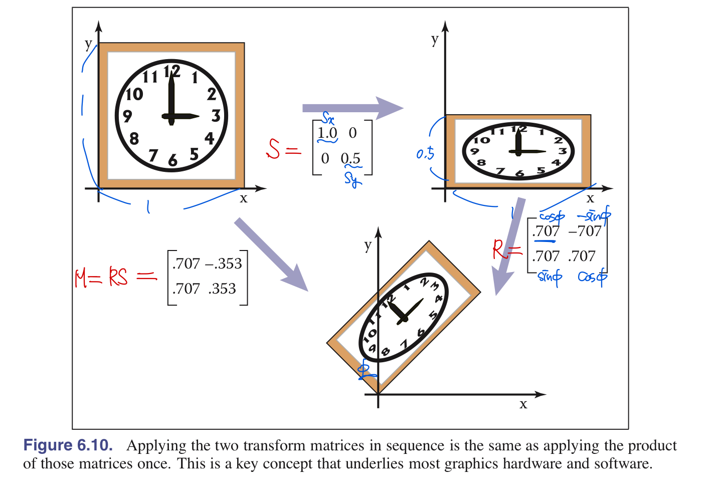
• 중요한 것은, 이러한 변환들은 오른쪽 변환부터 적용된다는 것을 혼동하면 안됨, 즉, RS에서 scaling먼저 적용하는 의미
• 이 순서가 바뀌면 결과도 달라짐

1.6. Decomposition of Transformations

• Compoisition말고 곱해진 상태의 변환 행렬을 “분해”하는 방법
• 크게 고유값 분해(Eigenvalue Deomposition) 기반과 특이값 분해(Singular Value Decomposition)기반 방법이 있다.
  

1. Symmetric Eigenvalue Deomposition

• 행렬이 symmetric(대칭)행렬일 때, \(\mathrm{A} = \mathrm{R}\mathrm{S}\mathrm{R}^T\) 으로 분해됨
  

  1) $\mathrm{R}^T$ 변환 : 행렬 A의 eigen vector(고유벡터)인 $\mathrm{v_1}$과 $\mathrm{v_2}$를 x 또는 y축 기반으로 회전시킴
  2) $\mathrm{S}$ 변환 : x와 y를 $(\lambda_1, \lambda_2)$만큼 scaling 시킴
  3) $\mathrm{R}$ 변환 : $\mathrm{v_1}$과 $\mathrm{v_2}$를 x 또는 y축 기반으로 다시 역회전시킴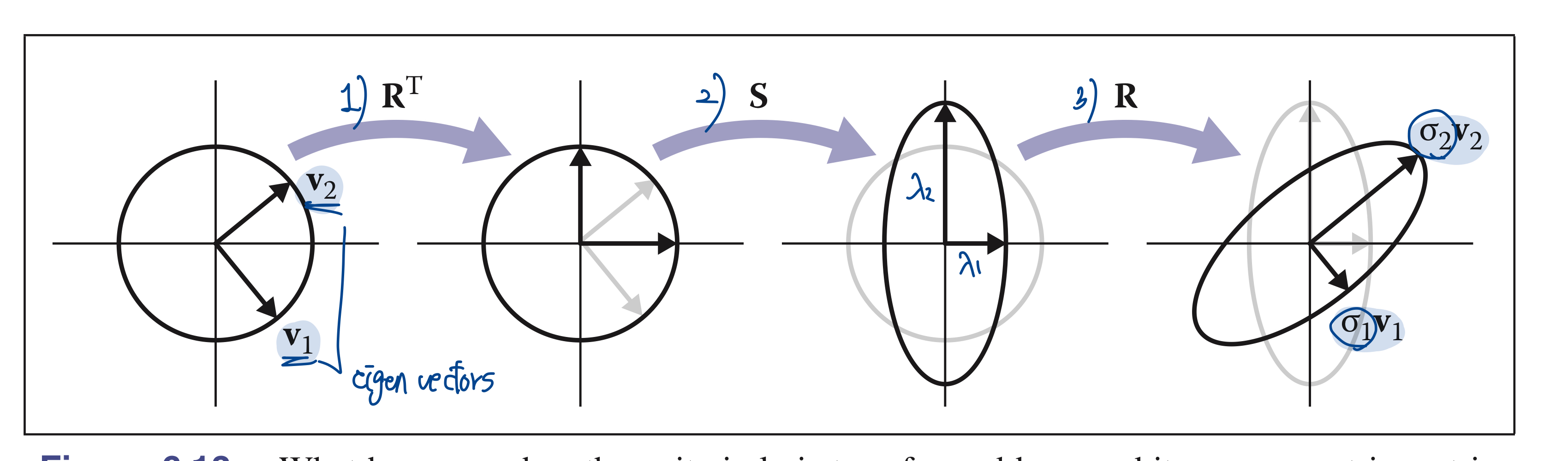

2. Singular Value Deomposition

• 전체적으로 과정은 같음, 대신 전체 변환행렬 A가 대칭행렬이 아님
• 고유값 대신 특이값사용

2. 3D Linear Transformations

• 2D 변환의 확장된 ver.

3. Translation and Affine Transformations

[1] 변환 행렬 M이 곱해졌을 때,

\[\begin{align} x' = m_{11}x + m_{12}y \\ y' = m_{21}x + m_{22}y \end{align}\]

[2] Translation 이 있을 때,

\[\begin{align} x' = x + x_t \\ y' = y + y_t \end{align}\]

위의 두 가지 변환 연산을 합친 Transformation matrix M을 single하게 어떻게 나타낼 것인가,
trick : Homogeneous coordinate을 이용함 : $(x \quad y) -> [x \quad y \quad 1]^T $

\[M = \begin{bmatrix} m_{11} & m_{12} & x_t \\ m_{21} & m_{22} & y_t \\ 0 & 0 & 1 \end{bmatrix}\]

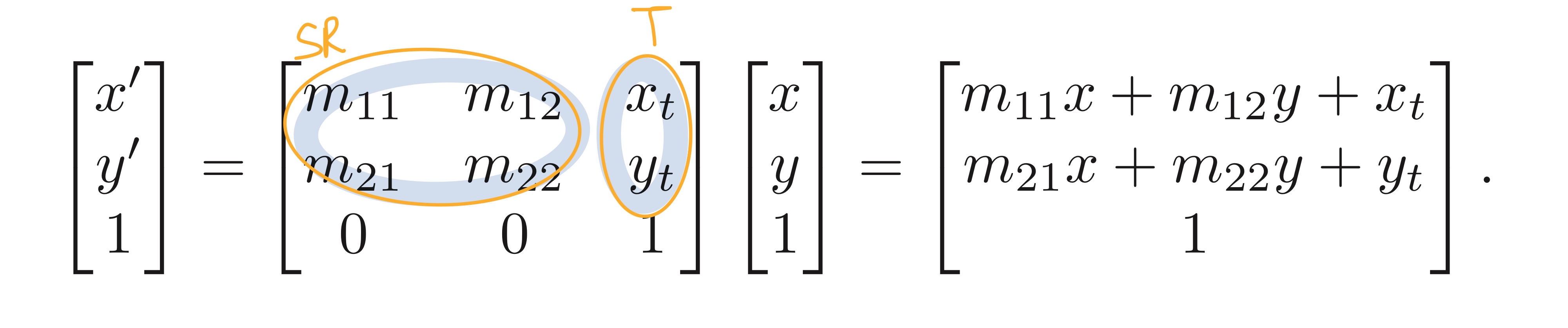
이렇게 곱해지는 형태의 변환을 “Affine Transformation” 이라고 한다.

… 이어서